1. Leaf Area Index related parameters
Necessary packages for analysis:
[1]:
import pandas as pd
import numpy as np
import matplotlib.pyplot as plt
from datetime import datetime
from pathlib import Path
import supy as sp
import os
from shutil import copyfile
import geopandas as gpd
import pickle
pd.options.mode.chained_assignment = None
from IPython.display import clear_output
import warnings
warnings.filterwarnings('ignore')
This is a custom package specifically designed for this analysis. It contains various functions for reading and computing and plotting.
[2]:
from alb_LAI_util import generate_array_dif, generate_array_same, modify_attr,func_parse_date
1.1. Parameters needed to calcuate LAI for non-crop vegetation (see Background https://umep-workshop.readthedocs.io/en/latest/Parameters/CalcBG.html)
- \(BaseT\) -
- \(BaseTe\)
- \(LAI_{MAX}\)
- \(LAI_{Min}\)
1.2. Necessary functions for analysis
1.2.1. Read in the data (including LAI data)
[3]:
def read_data(year, name):

    df = pd.read_csv('data/MODIS_LAI_AmeriFlux/statistics_Lai_500m-' + name +
                     '.csv')
    if name!='crop':
        df.columns = ['product'
                      ] + [i.split(' ')[1] for i in df.columns if i != 'product']

    df = df.filter(['modis_date', 'value_mean'])

    df_period = df[[i.startswith('A' + str(year)) for i in df.modis_date]]
    df_period.loc[:, 'DOY'] = [
        int(i.split('A' + str(year))[1]) for i in df_period.modis_date
    ]
    df_period = df_period.set_index('DOY')

    copyfile("./runs/data/" + name + "_" + str(year) + "_data_60.txt",
             "runs/run/input/Kc_2012_data_60.txt")
    df_forcing = pd.read_csv('runs/run' + '/Input/' + 'kc' + '_' + '2012' +
                             '_data_60.txt',
                             sep=' ',
                             parse_dates={'datetime': [0, 1, 2, 3]},
                             keep_date_col=True,
                             date_parser=func_parse_date)

    all_sites_info = pd.read_csv('site_info.csv')
    site_info = all_sites_info[all_sites_info['Site Id'] == name]
    df = pd.DataFrame({
        'Site': [name],
        'Latitude': [site_info['Latitude (degrees)']],
        'Longitude': [site_info['Longitude (degrees)']]
    })

    path_runcontrol = Path('runs/run' + '/') / 'RunControl.nml'
    df_state_init = sp.init_supy(path_runcontrol)

    df_state_init ,level= modify_attr(df_state_init, df, name)

    grid = df_state_init.index[0]
    df_forcing_run = sp.load_forcing_grid(path_runcontrol, grid)

    df_output, df_state_final = sp.run_supy(df_forcing_run,
                                            df_state_init,
                                            save_state=False)

    return df_output, df_state_final, df_state_init, df_period, grid, df_forcing_run,level
1.2.2. Calculating some of the variables of the models (LAI,GDD,SDD,Tair)
[4]:
def calc_vars(df_output, grid, df_forcing_run,year,level):

    df_output_2 = df_output.loc[grid, :]
    df_output_2 = df_output_2[df_output_2.index.year >= year]

    lai_model = pd.DataFrame(df_output_2.SUEWS.LAI)
    a = lai_model.index.strftime('%j')
    lai_model['DOY'] = [int(b) for b in a]

    if(level==1):
        nameGDD='GDD_DecTr'
        nameSDD='SDD_DecTr'
    elif(level==0):
        nameGDD='GDD_EveTr'
        nameSDD='SDD_EveTr'
    if(level==2):
        nameGDD='GDD_Grass'
        nameSDD='SDD_Grass'

    GDD_model = pd.DataFrame(df_output_2.DailyState[nameGDD])
    a = GDD_model.index.strftime('%j')
    GDD_model['DOY'] = [int(b) for b in a]
    GDD_model = GDD_model.dropna()
    GDD_model = GDD_model.iloc[1:]

    SDD_model = pd.DataFrame(df_output_2.DailyState[nameSDD])
    print(SDD_model)
    a = SDD_model.index.strftime('%j')
    SDD_model['DOY'] = [int(b) for b in a]
    SDD_model = SDD_model.dropna()
    SDD_model = SDD_model.iloc[1:]

    Tair = df_forcing_run.Tair.resample('1d', closed='left',
                                        label='right').mean()
    Tair = pd.DataFrame(Tair)
    a = Tair.index.strftime('%j')
    Tair['DOY'] = [int(b) for b in a]

    return lai_model, GDD_model, SDD_model, Tair,nameGDD,nameSDD
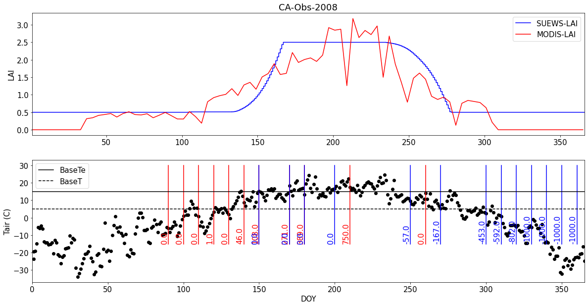
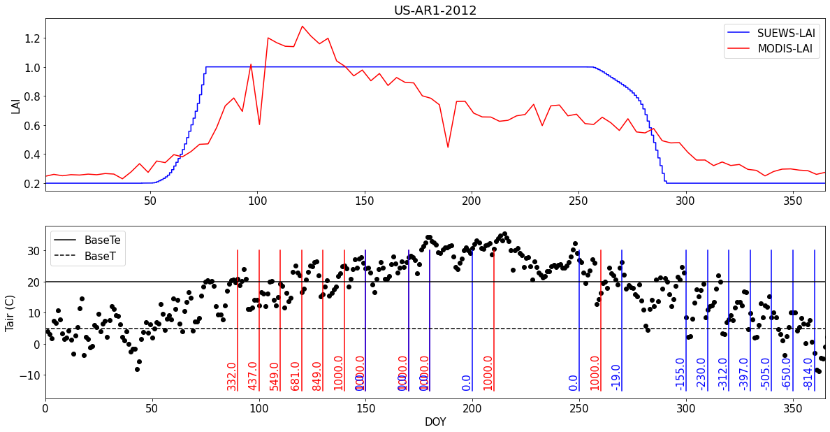
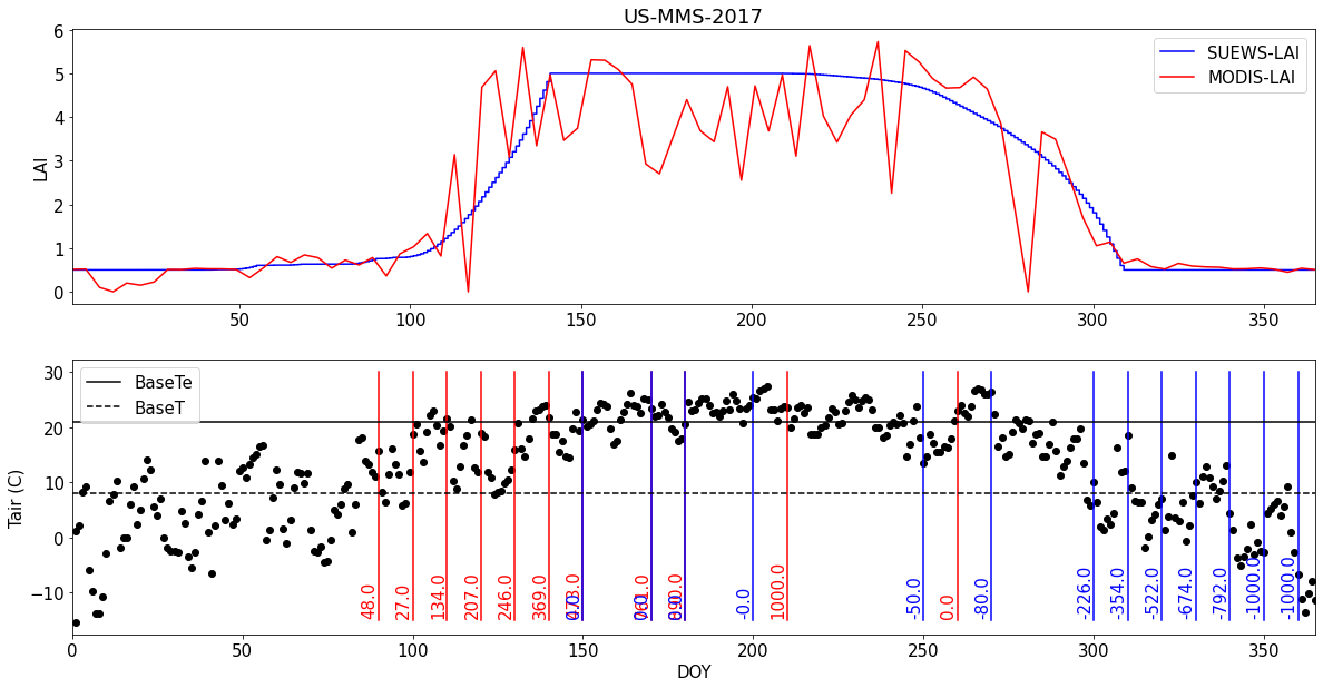
1.2.3. Calculate and plot the LAI for the site being analysed. The data are saved to a pickle file.
[5]:
def LAI_tune(year,name):
    df_output,df_state_final,df_state_init,df_period,grid,df_forcing_run,level = read_data(year,name)
    lai_model,GDD_model,SDD_model,Tair,nameGDD,nameSDD=calc_vars(df_output,grid,df_forcing_run,year,level)
    clear_output()

    with open('outputs/LAI/'+name+'-'+str(year)+'-MODIS.pkl','wb') as f:
        pickle.dump(df_period, f)
    with open('outputs/LAI/'+name+'-'+str(year)+'-Model.pkl','wb') as f:
        pickle.dump(lai_model, f)

    attrs=[
    df_state_init.loc[:,'laimin'].loc[grid][level],
    df_state_init.loc[:,'laimax'].loc[grid][level],
    df_state_init.loc[:,'basete'].loc[grid][level],
    df_state_init.loc[:,'baset'].loc[grid][level]
    ]

    with open('outputs/LAI/'+name+'-attrs.pkl','wb') as f:
            pickle.dump(attrs, f)

    plt.rcParams.update({'font.size': 15})
    fig,axs=plt.subplots(2,1,figsize=(20,10))
    ax=axs[0]
    ax.plot(lai_model.DOY,lai_model.LAI,color='b',label='SUEWS-LAI')
    df_period.value_mean.plot(color='r',label='MODIS-LAI',ax=ax)
    ax.set_ylabel('LAI')
    ax.legend()
    ax.set_title(name+'-'+str(year))
    ax.set_xlabel('')

    ax=axs[1]
    plt.scatter(Tair.DOY,Tair.Tair,color='k')


    try:
        max_y=30
        for gdd_day in [90,100,110,120,130,140,150,170,180,210,260]:
            a=GDD_model[GDD_model.DOY==gdd_day][nameGDD]
            plt.plot([gdd_day,gdd_day],[-15,max_y],color='r')
            plt.annotate(str(np.round(a.values[0],0)),(gdd_day-5,-14),color='r',rotation=90)


        for sdd_day in [150,170,180,200,250,270,300,310,320,330,340,350,360]:
            a=SDD_model[SDD_model.DOY==sdd_day][nameSDD]
            plt.plot([sdd_day,sdd_day],[-15,max_y],color='b')
            plt.annotate(str(np.round(a.values[0],0)),(sdd_day-5,-14),color='b',rotation=90)
    except:
        pass

    ax.plot([0,365],[df_state_init.basete.iloc[0][0],df_state_init.basete.iloc[0][0]],label='BaseTe',color='k')
    ax.plot([0,365],[df_state_init.baset.iloc[0][0],df_state_init.baset.iloc[0][0]],'--k',label='BaseT')
    ax.legend()
    plt.ylabel('Tair (C)')
    plt.xlabel('DOY')
    ax.set_xlim(left=0,right=365)
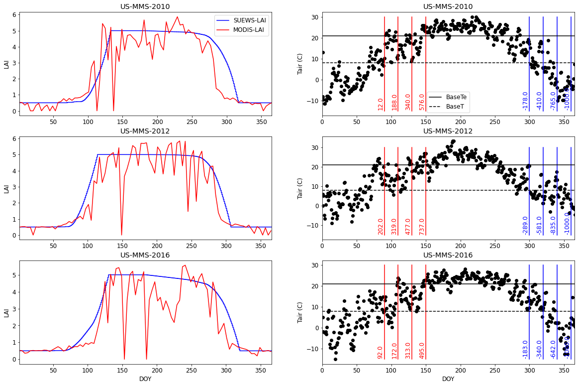
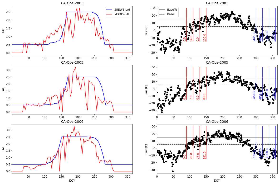
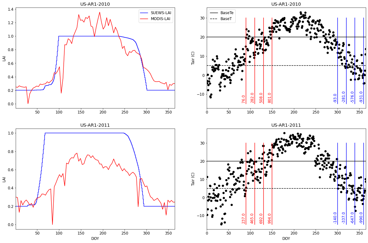
1.2.4. Now evaluate the LAI parameters at other ‘Test’ sites. Calculate and plot LAI (and save data to pickle files)
[6]:
def LAI_test(years,name):

    plt.rcParams.update({'font.size': 12})
    fig,axs=plt.subplots(len(years),2,figsize=(20,13))

    counter=-1
    for year in years:
        print(name+'-'+str(year))
        counter=counter+1
        df_output,df_state_final,df_state_init,df_period,grid,df_forcing_run,level = read_data(year,name)
        lai_model,GDD_model,SDD_model,Tair,nameGDD,nameSDD=calc_vars(df_output,grid,df_forcing_run,year,level)
        clear_output()

        with open('outputs/LAI/'+name+'-'+str(year)+'-MODIS.pkl','wb') as f:
            pickle.dump(df_period, f)
        with open('outputs/LAI/'+name+'-'+str(year)+'-Model.pkl','wb') as f:
            pickle.dump(lai_model, f)


        ax=axs[counter][0]
        ax.plot(lai_model.DOY,lai_model.LAI,color='b',label='SUEWS-LAI')
        df_period.value_mean.plot(color='r',label='MODIS-LAI',ax=ax)
        ax.set_ylabel('LAI')
        if counter==0:
            ax.legend()
        if counter!=len(years)-1:
            ax.set_xlabel('')
        ax.set_title(name+'-'+str(year))


        ax=axs[counter][1]
        ax.scatter(Tair.DOY,Tair.Tair,color='k')
        try:
            max_y=30
            for gdd_day in [90,110,130,150]:
                a=GDD_model[GDD_model.DOY==gdd_day][nameGDD]
                ax.plot([gdd_day,gdd_day],[-15,max_y],color='r')
                ax.annotate(str(np.round(a.values[0],0)),(gdd_day-10,-14),color='r',rotation=90)


            for sdd_day in [300,320,340,360]:
                a=SDD_model[SDD_model.DOY==sdd_day][nameSDD]
                ax.plot([sdd_day,sdd_day],[-15,max_y],color='b')
                ax.annotate(str(np.round(a.values[0],0)),(sdd_day-10,-14),color='b',rotation=90)
        except:
            pass
        ax.plot([0,365],[df_state_init.basete.iloc[0][0],df_state_init.basete.iloc[0][0]],label='BaseTe',color='k')
        ax.plot([0,365],[df_state_init.baset.iloc[0][0],df_state_init.baset.iloc[0][0]],'--k',label='BaseT')
        if counter==0:
            ax.legend()
        ax.set_ylabel('Tair (C)')
        if counter==len(years)-1:
            ax.set_xlabel('DOY')
        ax.set_xlim(left=0,right=365)
        ax.set_title(name+'-'+str(year))

    plt.savefig('figs/'+name+'-LAI.png',dpi=300,bbox_inches = 'tight',pad_inches = 0.01)
1.3. Plot for all sites
1.3.1. DecTr
1.3.1.1. US-MMS
[7]:
name='US-MMS'
year=2017
LAI_tune(year,name)
[8]:
name='US-MMS'
years=[2010,2012,2016]
LAI_test(years,name)